An operator can be thought of as an entity which operates on a given function to give us another function. For example, in mathematics we have, say,
![]()
Here,
![]() is an operator which operates on f (x) to yield
f
is an operator which operates on f (x) to yield
f![]() (x).
(x).
In classical mechanics, to solve any problem we deal directly with physical properties or observables like position, momentum, energy etc.
In quantum mechanics, however, we work with operators corresponding to the respective physical observables. Each physical observable, therefore, has a corresponding linear, Hermitian operator in quantum mechanics. Â is a linear operator if
![\begin{eqnarray*}
{\hat {A}}[f_{1}(x)+f_{2}(x)] & = & {\hat {A}}f_{1}(x)+ {\hat {A}}f_{2}(x) \\
{\hat {A}}[k f(x)] & = & k{\hat {A}} f(x)
\end{eqnarray*}](elearningimg40.png) .
.
Again  is Hermitian if
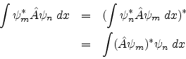
where ![]() and
and
![]() are any two wavefunctions.
are any two wavefunctions.
The above integrals may be written in a very compact way called Dirac bracket notation.
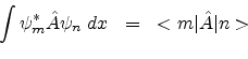
In this notation | n >, called ket n, represents the state of the system with wavefuction ![]() and | m >, called ket m, represents the state of the system with wavefuction
and | m >, called ket m, represents the state of the system with wavefuction ![]() .
.
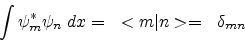
where ![]() is called the Kronecker delta symbol:
is called the Kronecker delta symbol:
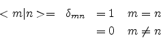
corresponding to the set of normalized wavefunctions or the set of orthogonal wavefunctions respectively.
In this notation, the condition for Hermiticity may be expressed simply as
In this context we may want to know what is an eigen-value equation.
![]()
The above equation is called an eigen-value equation. a is called the eigen-value of the operator  and f (x) is called the corresponding eigen function. We will encounter more such equations later on.
Quantum mechanical operators can be represented in different representations, like position representation, momentum representation etc. In the position representation each quantum mechanical operator corresponding to a physical observable O is obtained by going through the following steps:
* Write down the observable in terms of cartesian coordinates qi and the corresponding momenta pi.
* Replace each qi with the multiplicative operator ![]() .
.
* Replace each pi with the operator
![]()
In the momentum representation, on the other hand, each quantum mechanical operator corresponding to a physical observable O is obtained by going through the following steps:
* Write down the observable in terms of cartesian coordinates qi and the corresponding momenta pi.
* Replace each qi with the operator
![]()
* Replace each pi with the multiplicative operator ![]() .
.
We would be using the position representation for most purposes.
The Hamiltonian operator ![]() can be written as a sum of the kinetic and potential energy operators which in turn can be written as
can be written as a sum of the kinetic and potential energy operators which in turn can be written as
![]() and V respectively.
and V respectively.
![]() is called the Laplacian in 3-dimensional cartesian coordinates and
is called the Laplacian in 3-dimensional cartesian coordinates and ![]()
Substituting in the eigen-value equation
![]()
we have what is known as Schrodinger's time independent equation
E is called the eigen-value of
![]() and
and ![]() is the corresponding eigen-function.
is the corresponding eigen-function.